Lab 17 - Finding the Moment of Inertia of a Uniform Triangle about its Center of Mass

Purpose: To determine the moment of inertia of a triangle on a spinning base by using a hanging mass with known value, without having to calculate all of the individual moments of the separate pieces on the spinning base. Then compare with value for moment of inertia as calculated by using the parallel axis theorem.

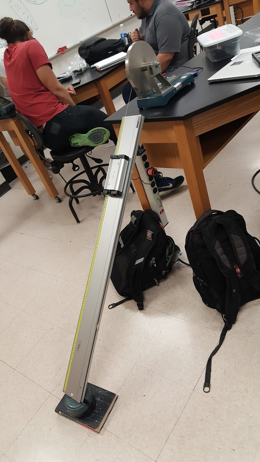
Apparatus:  The setup that we used for this lab is the same as the one that we used for lab 16, except the only difference is that above the pulley there was a mount for attaching a metal triangle with a hole through its center of mass.

Procedure: The procedure was simple, let the setup accelerate three times, and then record the up α and the down α, then take an average of the two. The three setups were as follows:

1) The system was allowed to accelerate without the triangle on the mount/hinge.
2) The metal triangle was mounted on the hinge, with the short base parallel to the ground, then the system was allowed to accelerate.
3) The triangle was rotated 90 degrees so that the long base would now be parallel to the ground.

The specs for the triangle are:
Mass = 454.7g
Short base = 98.1 mm
Long base = 149.1mm

The hanging mass was 24.9g, and attached to a torque pulley of radius 0.01245m

The values for the angular acceleration were recorded through logger pro as always. The angular acceleration for the system without the triangle was needed in order to  calculate the moment of inertia for the system, then subtract it from the moment of the system with the triangle on it. This would then yield the moment of inertia of just the triangle.

Raw data:

My calculations for the moment of inertia around center of mass.

My calculations for the moments of inertia by experiment.

Theoretical moments of inertia.

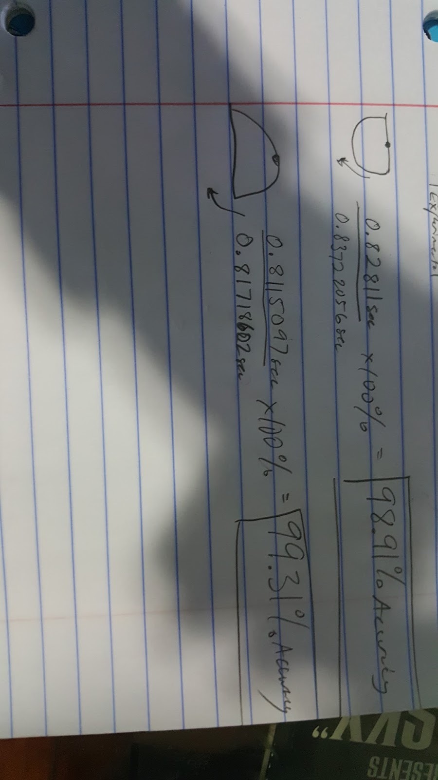
Percent Error:
At first the percent error for the short base and long base configuration was 48.7% and 50.0% respectively. This lead me to believe that I may have used the incorrect sized pulley for my calculations due to it being off by a factor of 2. After I made an adjustment by multiplying the experimental values by 2, the error changed to 2.65% for the short base and 0.065% for the long base.

Conclusion:  Assuming that all my calculations are correct, I think that this lab went well. However, I do regret taking so long to write up this lab because as with all the other experiments, after writing up the lab I have a much more solid understanding of the concepts we are studying. Not only do I have solid understanding of how moment of inertia is just a value for the mass distribution about a radius, but now I understand the parallel axis theorem better. However, I do not understand how the theoretical value for the triangle with the longer base is larger than the experimental value. This makes no sense because the theoretical value is assuming that the system does not have friction in it.

My lab partners were Mia and Jarrod.

Lab 16 - Angular Acceleration

Purpose: To study how different factors affect the values for angular acceleration and moment of inertia. Then calculate values for the moment of inertia for different masses.

Apparatus: The setup that we used was a tabletop where metal disks can sit atop an axis of rotation that has compressed air flowing through it. The compressed air helps to reduce the amount of friction in the system and allows the metal disks to "float" freely about the axis. There are two disks, one steel one at the bottom and either a steel one on top, or an aluminum one on top. At the top of the stacked disks is a threaded hole where we were able to attach pulleys of varying sizes. The pulley then had a string with a hanging mass attached to it. The hanging mass was then hung off the edge of the table and let go in order to allow the system to accelerate. The string came off the disks horizontally, then changed direction to be vertical by way of another small, free-rotating pulley of negligible mass. The two larger metal disks each had 200 vertical stripes in order for a sensor on the setup to read how fast the disk was spinning. The data was then reported on a graph on logger pro.

Procedure: First thing I did was measure out all the diameters and masses of the disks, pulleys, and hanging mass.

Diameter and Mass
Top steel disk = 126.4mm, 1359g
Bottom steel disk = 126.4mm, 1347g
Top aluminum disk = 126.3mm, 466g
Small torque pulley = 24.9mm, 10.1g
Large torque pulley = 49.7mm, 36.1g
Hanging mass = 25.0 g

Comparisons: (Approximate ratios)
1) Ratio of small pulley to large pulley= 1:2
          Ratio of angular accelerations = 1:2
2) Hanging mass ratio 25g/50g = 1:2
          α = 1:2
3) Hanging mass ratio 25g/75g 1:3
          α = 1:3
4)Mass of top steel disk/mass of top aluminum = 3:1
          α = 1:3
5)Mass of top steel disk/top steel+bottom steel = 1:2
          α = 2:1
6) Diameter of small pulley/diameter of large pulley = 1:2
          α = 1:2

Experimental Angular accelerations:
1) 25g hanging mass, small pulley,top steel disk. Average α = 0.62295 rad/s/s

2) 50g mass, small pulley, top steel disk. Average α = 1.2495 rad/s/s

3) 75g mass, small pulley, top steel disk. Avg α = 2.259 rad/s/s

4) 25g mass, large pulley, top steel disk. Avg α = 1.2175 rad/s/s

5) 25g mass, large pulley, top aluminum.  Avg α = 3.4095 rad/s/s

6) 25g mass, large pulley, top+bottom steel disks. Avg α = 0.6109 rad/s/s

 This picture above shows all my calculations for the experimental moments of inertia for all of the disk combinations.

Conclusion: What I learned from my calculations of the moments of inertia are that although the angular acceleration can vary due to many factors such as radius, or torque, the moment of inertia still remains constant. This is important because it helped me see the connection between F=ma and T=Iα.
The moment of inertia remains constant in the experiments where the disk is the same, which is to be expected because the mass does not change just because it is being accelerated faster. The only thing that is different between a mass and a moment of inertia is that a moment of inertia takes into account the distribution of that mass along a radius. Some sources of error in this lab are the fact that none of these surfaces were frictionless, so we may have gotten smaller numbers for α, which meant that the moment of inertia was too large since we were dividing by α. Another source of error was that I was working alone with no lab partners for this experiment. Lastly, one more source is error is the fact that trying to get the right flow of compressed air through the system was kind of tricky, so it may or may not have skewed our results.

Lab 18 - A Lab Problem- Moment of Inertia and Frictional Torque

Purpose: To predict the time for a cart on a downward-angled track to descend 1meter at a 40 degree incline, that is tied by a light string to a large metal disk that will spin as the cart descends. We will do this by first calculating frictional torque for the heavy metal disk.

Apparatus: A large, heavy metal cylinder on a lathe-like stand with known mass, and unknown moment of inertia. A cart-track is angled down off the edge of the lab table at a 40 degree angle with the horizontal. A cart is tied to a light string, which is then wound around the smaller diameter of the large disk, which will exert a torque on the disk as the cart descends down the ramp a distance of 1meter.

Procedure: We first started by calculating the frictional torque of the large disk by placing a piece of tape on the large disk, somewhere around the outer diameter and marking it with a dot. Then we recorded a video while it spun, and slowed down with friction in its own axis. We then used logger pro to pinpoint the location of the dot as it went around in a circle. We then plotted linear velocity vs. time to get a linear acceleration (deceleration). After we figured out a linear acceleration, it was easy to find α by simply dividing the linear acceleration by the radius from the axis of rotation to the dot.

Below is a picture of the whiteboard where we recorded all of the dimensional information for the wheel as we measured it. The total mass was stamped on the wheel, which was 4.862kg. After we summed up all of the volume for the different sections of the wheel, we used ratios of volume/total volume = mass of section/total mass to figure out how much each piece of the wheel weighed. This is because the wheel was a large disk, with a smaller diameter cylinder protruding out the sides through the axis of rotation, so each piece has a different moment of inertia.

 After calculating how much mass is distributed to the cylinders and to the disk, it was pretty straight-forward to calculate the moment of inertia of each piece. Then, the moments were summed up in order to know the moment of inertia for the wheel as a single piece.

 Frictional torque  = Iα
α = derived from the video earlier on logger pro.

This is a picture of the apparatus all put together in the end. Most of the time was spent calculating the frictional torque for the metal disk in order to accurately calculate the predicted time of descent.

Trial 1: 10.22 sec
Trial 2: 10.85 sec
Trial 3: 10.07 sec

Average: 10.36 sec

 Theoretical: 10.43 sec

Percent Error: 0.70%

 Below are my calculations for the theoretical time of descent.

Conclusion: In this lab I learned that any object that is spinning has some kind of frictional torque. This is because if there wasn't, the object would just keep spinning forever and that is impossible. I learned that I can express the amount of friction inside a spinning system as a torque value. This is important because this makes it fairly easy to calculate how friction inside a rotating assembly will affect the motion of other things in the system. I was a little weird to see that our average value for the time it took the cart to travel 1m was smaller than the theoretical. This could be due to many reasons, one being human error. There is much room for error when timing the cart to descend 1 meter because certain things such as reaction time for the stopping and starting of the stopwatch can vary from person to person, and even trial to trial. Another reason is that we calculated the frictional torque and ran the trials on two separate days. On the second day we noticed that the wheel had started to squeak, which probably indicated that for one reason or another (maybe more moisture in the room), there may have been slightly different values for the frictional torque. It was pretty cool to be able to relate linear kinematics with rotational kinematics and rotational friction. 

My lab partners were Mia and Jarrod.

Lab 19 - Conservation of Energy/Conservation of Angular Momentum

Purpose: To use conservation of angular momentum and angular kinetic energy to predict how high a swinging meter stick will go after colliding inelastically with a piece of clay sitting on the ground.

Apparatus: We used a clamp to hold a sensor that is normally for logger pro for measuring angle(maybe?), except we just used the sensor as an axis of rotation because it was relatively simple to attach a meter stick to. The meter stick had a hole at the 0.015m mark,  and this is where we threaded a screw through in order to make the meter stick swing about an axis. We then bent a paper clip into an asymmetrical shape in order to provide a little stand so that a piece of clay is not making contact with the ground, which reduces friction between the clay and the ground. This is important because if the clay drags on the ground after the meter stick swings down and catches it, much energy will be lost in the system to friction/thermal energy. We wrapped tape (sticky side out) around the meter stick and around a ball of clay. The tape was to make sure that this would be an inelastic collision.

Procedure:  Mass of meter stick = 0.1612kg                    Mass of clay = 0.0387kg

We lifted the meter stick to be horizontal, then let it go. It swung down and collided inelastically with a piece of clay with tape on the ground that was being held up by a paper clip, and we took a video of the whole incident from start to finish. We then uploaded to logger pro and analyzed how high the piece of clay rose in the direction of the y-axis.

Below are my calculations for the moment of inertia of the meter stick both before and after collision. There are two different moments of inertia because after collision, there is a "point mass" rotating about an axis. This point mass is the piece of clay that sticks onto the ruler. In the calculations below, we had to use 1/12mr^2 with a parallel axis shift instead of 1/3mr^2 because the axis of rotation is not exactly at the edge of the ruler, and the parallel axis shift only works with the moment around a center of mass. We then set GPE=Rot. KE to find the value for ω at the bottom of the swing. The GPE used half the height of the meter stick because gravity "acts" on the center of mass only.

Next, just like in linear collisions, we conserved angular momentum to find the new angular velocity after impact.
Lbefore=Lafter
Iω=Iω
Lafter takes into account the moment of inertia of the clay combined with the moment for the meter stick.

The scratch marks below are where I learned that I cannot simply equate the Rot.KE back to GPE to get a value because it was way off.

What we had to do was a little more involved, but no where near impossible. Instead of calculating the new center of mass for the meter stick-clay system, we separated the two different changes of height for the two centers of mass. We said GPE(clay)+GPE(cm ruler)= 1/2Iω^2.
 Then by similar triangles, or a proportion of the change in height of the centers of mass relative to the position along the ruler they were at, to the axis of rotation, we came up with a way to eliminate one unknown variable. This made it possible to solve the equation for a single variable which was the change in height of the piece of the clay. We chose to solve for this center of mass because it was much more easier to pinpoint the position of the clay on logger pro as opposed to the center of the meter stick.

Theoretical height = 0.38246m

The picture above shows the maximum height of the clay after impact.
Max height = 0.3541-0.0001197= 0.3539803m

Percent error = 7.45%

The amount in error in this experiment is not because we did something wrong. It is because there are factors that contribute to significant error in this lab. Some of these errors include the fact that no matter how many times we tried, we could not get the collision to happen without the clay catching some friction on the ground, which uses up KE to create thermal energy. Another source of error in this lab is that mapping the position of the clay on logger pro is not very precise. This creates error because clicking a tiny bit off from the intended position on the video causes the data to be off by a magnified amount.

Conclusion: It is pretty cool to see that many of the same principles for linear calculations still apply in rotational bodies. Also, I learned that although calculations are a little more involved, they are fairly straight-forward. I have a better sense of understanding of the physical world around me and can see that in a collision, to calculate everything I need to break things up into phases. I think I have a pretty solid understanding of collisions after this lab, including collisions with rotating objects. I learned that if things stick together, momentum (whether linear or rotational) must be conserved because a "new" object with a different mass, which changes the velocity of the system. Then, energy can be "conserved" in an equation, but if you equate it back to GPE, you must find the center of mass for it to be valid.

Lab Partners:
Haokun Zhang
Christian Rivera

Lab 20 - Conservation of Linear and Angular Momentum

Purpose: To make a connection between conservation of linear momentum and angular momentum through torque mechanics and moment of inertia.

Procedure: A ball was rolled down a ramp of known height, ball collided in-elastically with a perpendicular arm rotating about an axis. We found a value for the angular acceleration of the system with logger pro, and used it to find the value for the moment of inertia of the system. With the mass of the ball, velocity, and distance of impact from the axis of rotation, we were able to predict with good accuracy the angular speed of the system after impact. We were able to do this by relating the linear momentum of the ball to the angular momentum of the system.

The picture below shows how we determined the final velocity of the metal ball as it leaves the bottom of the ramp. This method is similar to how we measured the muzzle velocity of the cannon/gun in the "ballistic pendulum" lab. We positioned the ramp at the edge of the table, measured a vertical distance to establish a relationship with time, and a vertical distance to divide by the time the ball spends in the air to figure out the horizontal velocity.

Vf=1.35m/s.
Mass of ball = 0.0289kg
radius of ball = 0.0095m

Below are my calculations for the horizontal velocity of the ball as it leaves the ramp. (sorry for orientation of photo)

This picture below is of the setup. We hung a mass of 0.0246kg off of a pulley of radius 9=(0.0499/2)meters. The angular acceleration was then measured through logger pro and we found the average  angular acceleration to be 5.6305rad/s/s.
We then equated torque to I*(alpha)
F*d=Iα
F=mg=0.0246kg*9.8m/s/s
d=(0.0499/2)m
α=5.6305rad/s/s
I=(after solving)=0.00105kgm^2

This is a graph of the raw data after the hanging mass was let go, and the two values from which we calculated an average value for the angular acceleration are shown on the two squares towards the bottom.

This is a closer picture of the apparatus that we used to demonstrate the conservation of linear and angular momentum. You can see the ramp where the ball comes down, and collides with a perpendicular arm that also grabs the ball once it comes down. The mass of the ball affects the overall moment of inertia due to it becoming a part of a rotating mass once the inelastic collision takes place.

More Calculations:

The picture above shows two different trials in which we predicted a quantity for ω.
Trial 1: The ball impacted at a right angle, and a distance 0.076m from the axis of rotation. We then used a similar equation to the one from before:         m*v*d=Iω
 "I" of the system had to be recalculated, which was just the one we calculated earlier, plus the moment for the ball+a parallel axis shift(which was equal to the distance from the center of the impact, to the axis of rotation).
I= 0.00105+(0.0289*0.076^2)+(0.0289*0.0095^2)*(2/5)
Distance from center of ball to axis of rotation = 0.076m

Experimental ω = 2.269 rad/s (as reported by logger pro)
Theoretical ω = 2.434 rad/s (as calculated)
Percent error: 6.78%  Error

Trial 2:
I= 0.00105+(0.0289*0.042^2)+(0.0289*0.0095^2)*(2/5)

Distance from center of ball to axis of rotation = 0.042m

Experimental ω = 1.353 rad/s
Theoretical ω = 1.487 rad/s
Percent error: 9.01% Error

Conclusion: It is pretty cool to see that the only thing that is needed to relate linear and angular momentum is a radius for the linear momentum. Like other relationships between linear and angular quantities, such as velocity and acceleration, all that is needed is a radial quantity to relate angular and linear momentum. This is important because it shows that in this physical universe, different quantities can be equated relatively simply. A collision at half the radius of another collision will result in a quarter the angular momentum being transmitted. This is because of the parallel axis shift, which is related by the distance from the pivot-squared. Since m*v*r=Iω, the relationship between the angular momentum and the horizontal velocity of the ball is linear because the velocity is not squared in the relationship. The relationship between the angle of impact is related by a quantity of sin Θ, because only the perpendicular component transmits any momentum from linear to angular.
I learned that linear momentum times a distance = angular momentum.

Lab Partners:
Haokun Zhang
Christian Rivera

Lab 21 - Mass-Spring Oscillations Lab

Purpose: To prove that the equation for period(below) is true.
T=2Pi*Sqrt(m/k)

Theory: The period of a mass-spring system can be predicted by a formula that is derived from Newton's 2nd law.

Procedure: Each group was assigned one spring of unknown spring constant. All of the springs had varying spring constants. We were assigned spring #5. We hung a spring off of a rod attached to the edge of the lab table, and measured the equilibrium position with respect to the ground. We then hung a mass on the spring, measured the change in distance and used F=kx to find the spring constant which turned out to be 29.4 N/m. We then took 1/3 of the mass of the spring which was 0.008kg, and the mass of the hook on the spring (0.0037kg), and used that information to find the mass that we needed in order to hang an exact mass of 0.115kg. The entire class did this in order to generate a table and graph for which the mass was held constant in the system, and the spring constants were varied.

0.008+0.0037+m=0.115kg
m=hanging mass needed

We then positioned a laptop right in front of the apparatus and set it to record oscillations of the spring system and we then used logger pro to measure the start and end of 10 oscillations. We then calculated the period for our spring with varying masses. We then plotted out the data.

Period v. Spring Constant for masses constant, varying spring constants

Period vs. Oscillating Mass

Below are percent error calculations for the periods that were measured in lab. The picture below shows the calculations for the first part, where we kept the hanging masses constant. For some reason, our group had the most error out of any other.

After calculating the percent errors for the second part, where we varied the masses, I noticed that we clearly had a systematic error somewhere in our experiment. As it turns out, what I believe that happened is that there was one extra oscillation in our calculations that we did not account for. When I applied a correction of (10/11), or percent errors jumped down by a lot. I do not believe that the error came from anywhere else because we were very careful, but maybe we did not start counting the oscillations from zero, which threw off all of our values for the period.

Here is my derivation for an expression for the period of a mass spring system using Newton's 2nd law.

Conclusion: What I learned in this lab is that the equation for finding the period of an oscillating spring-mass system holds true, whether you change the spring constant or the hanging mass. Also, I learned that it does not matter how much you stretch a spring before you release it into oscillation because the period will not change, the spring will just accelerate faster in order to compensate the extra distance. If the value of k was off by 5%, then the answer would be off by a factor of almost 25%. The period of a spring system should decrease if you increase the spring constant because the spring will be able to provide a larger force to an object. Using F=Ma, we can see that the acceleration will be much larger and thus, a smaller period. The period of a spring system will increase if you increase the oscillating mass by the same formula, because the acceleration will be smaller if you divide a force by a larger mass.

Lab 22 - Physical Pendulum Lab

Purpose To derive expressions for the period of differently shaped pendulums of varying mass and compare them to actual measured periods.

Apparatus: The apparatus was simple, a ring stand clamped to the lab table as shown below. The lower part of the ring stand had a photogate clamped onto it and was used to measure the period on logger pro. The first pendulum was a metal ring of mass 0.7519kg of outer radius .1465m and inner radius 0.1372m. However the ring was hung off an indentation that shifted the radius of the pendulum over by the average of the inner and outer radius, which turned out to be 0.14185m

Procedure: We first started by calculating the moment of inertia for every different shape. After we found the moments of inertia for the different pendulums, we then used torque equations to calculate the theoretical period for the oscillating pendulums. We used mgsin(theta)xRadius=I(alpha) and solved for alpha. After we solved for alpha, then we were able to solve for omega squared. When we divide 2Pi by omega, then we got the period.

 

Below are my calculations for the period of the hoop. Also included in the calculations are the %accuracy, which meant .07% error. This small amount of error in an experiment with limited technology is pretty amazing.

 The picture above shows the raw data on logger pro from the photogate for the hoop. The picture below was where we took the period information and took an average of it all.

 The next pendulum that we used was the semicircle supported  at the midpoint at the base.
I do not have the mass because I knew it would cancel out in the calculations, which I also told my lab partners we did not need. However, in retrospect it is very unprofessional of me to do so. I assume full responsibility for this; if my lab partners did not get the mass of the pendulum, I wish to be penalized for it alone because it was my fault.

Below are my calculations for the moment of inertia at the midpoint of the base, and the location of the center of mass.

 

The picture above is  of all the raw data put together to generate an average value.

 Avg= 0.83722056 sec

This picture below is of the raw data for the same pendulum, except we flipped it upside down. I completely forgot to take a picture of it before we took it down.

 This is the raw data put together to calculate an average value. Avg= 0.81718602 sec

 

Below are the calculations for the period of the semicircular pendulum with the pivot at the top.

 

Below are the % accuracy values for the semi-circle oriented two different ways.

 Below are the calculations for the moment of inertia around the center of mass for the semicircle, which were used for the parallel axis shifts. Also in this picture are the calculations for the moment around the top of the semi-circle.

 The two following pictures are my calculations for the triangular pendulum. Unfortunately, they are not very accurate.
:(

Conclusion: All in all I am actually pretty amazed at the accuracy of the period of the pendulums compared to the theoretical periods. All of the periods were within less than 1% error, which is unheard of for many lab experiments. The paper clips are located at the pivots for the semi-circular pendulum, and one on each side. The paper clips should not affect the moment of inertia because most of the mass is being supported by the hinge, and either way it would only add 1/3mr^2 for each of the clips. Compared to the rest of the pendulum, the mass and radius of the clips is very tiny. However, the tape has a larger effect on the moment of inertia because the piece used to mark the photogate is positioned at the furthest point on the pendulum. This would act as a point mass, which is mr^2, and this time the radius is actually much larger because it is at the outermost portion of the pendulum. I learned from this lab that pendulums are a much more accurate way to measure the value of gravity than a kinematics approach could ever be.

Lab Partners:
Haokun Zhang
Christian Rivera